When Does LeJEPA Learn a World Model?

Abstract

A representation that scrambles the true degrees of freedom of the world cannot support reliable planning or compositional generalization. We prove that LeJEPA (alignment plus Gaussian regularization) linearly recovers the world's latent variables from nonlinear observations — a property known as linear identifiability — in a broad class of worlds where latents evolve under stationary, additive-noise transitions. Our main result is that among all such worlds, the Gaussian is the unique latent distribution for which this guarantee holds. The forward direction rests on a spectral decomposition in which each degree of nonlinearity is strictly penalized by alignment, making the linear map the optimum; the converse rules out every non-Gaussian alternative. We further prove an approximate identifiability result where the guarantee degrades gracefully, and show that linear, orthogonal identifiability enables optimal latent-space planning. We validate the theory across 2D examples to 1024-dimensional latents, distributional ablations, and pixel-based robotic control. All theorems are formally verified in Lean 4.

TL;DR: LeJEPA linearly recovers the world's latent variables — up to rotation — if and only if those latents are Gaussian. The forward direction is a spectral argument on Hermite polynomials; the converse rules out every non-Gaussian alternative. All proofs are checked in Lean 4.

The Setup

LeJEPA learns the World Model — three-panel illustration

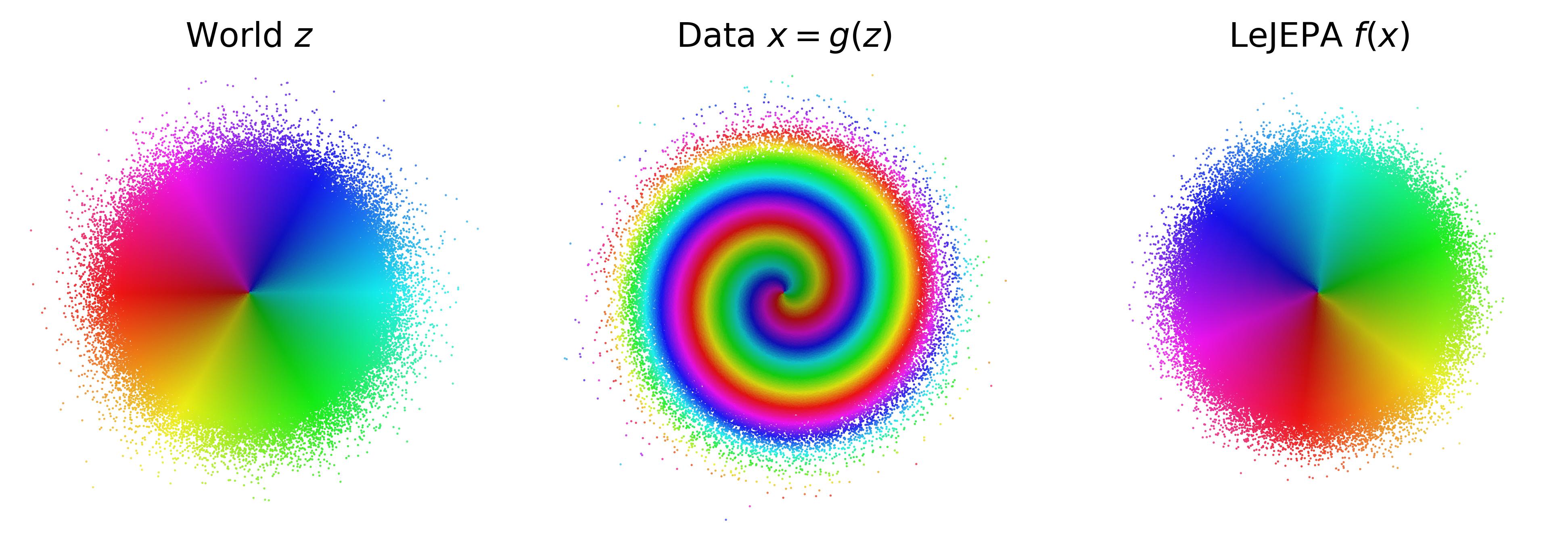
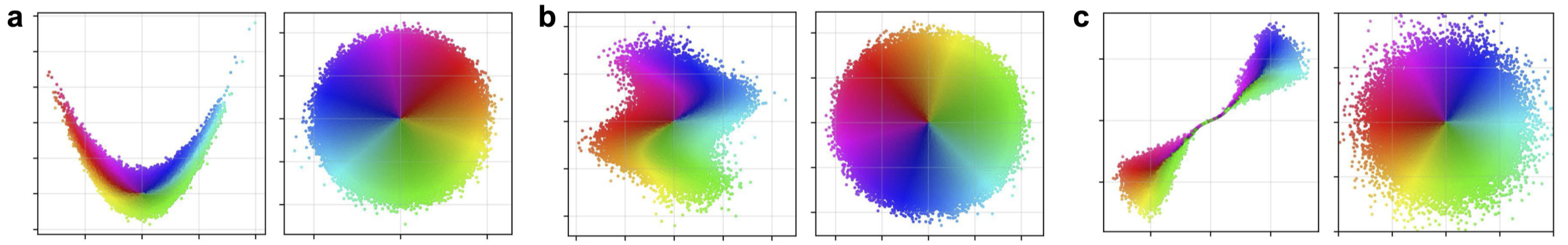
(left) The world has independent Gaussian latent variables. (center) An unknown nonlinear process scrambles them into the data we observe. (right) LeJEPA recovers the latent variables up to rotation. We prove this is the unique optimum.

The world. Latent variables $z \in \R^n$ with independent components and a stationary, additive-noise transition $z' = m(z) + \eta$. The world is observed through an unknown nonlinear mixing $x = g(z)$.

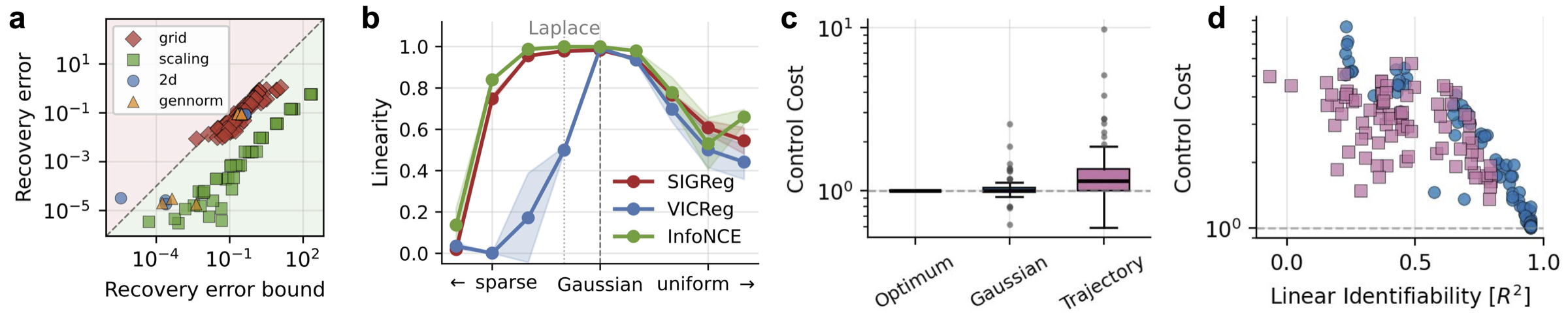
The learner. LeJEPA trains an encoder $h$ to minimize alignment between positive pairs $(z, z')$ subject to a Gaussianity constraint on its embedding distribution:

$$\min_h\ \E\!\left[\,\|h(z') - h(z)\|^2\,\right] \quad \text{s.t.} \quad h(z) \sim \N(0, I_n).$$

The Gaussianity constraint is enforced in practice by the Sketched Isotropic Gaussian Regularizer (SIGReg).

Theoretical Results

Theorem 1 — Forward Direction (Linear Identifiability)

For a Gaussian world, any $h$ that satisfies the Gaussianity constraint and minimizes alignment must be a rotation: $h(z) = Qz$ for some orthogonal $Q \in O(n)$. The proof rests on the Hermite-polynomial decomposition of $h$ under the Gaussian measure: every nonlinear component contributes strictly less to the temporal correlation than a linear one, so the optimum is linear.

Theorem 2 — Converse (Gaussian Uniqueness)

Within the class of stationary, additive-noise worlds, the Gaussian is the unique latent distribution under which LeJEPA achieves linear identifiability. Any non-Gaussian alternative breaks the recipe.

Theorem 3 — Approximate Identifiability

When the alignment and Gaussianity objectives are only $\varepsilon$- and $\delta$-close to satisfied, linear identifiability degrades continuously: the deviation from rotation is bounded by an explicit function of $(\varepsilon, \delta)$.

Theorem 4 — Optimal Latent-Space Planning

For any finite-horizon control problem whose costs are $O(n)$-invariant, the optimal value function and optimal action sequence in the learned latent space exactly equal those in the true latent space. Linear identifiability is therefore enough to plan optimally without ever recovering the latents themselves.

All four results are formally verified in Lean 4 with Mathlib (8,032 build targets, zero sorry obligations). Axiomatized components are standard background lemmas not yet in Mathlib (Hermite polynomial infrastructure, Mazur–Ulam, AM–GM with uniform weights).

Empirical Validation

2D illustrations. The teaser above already showed one mixing (a measure-preserving spiral). Below we test three more — parabolic shear, sinusoidal shear, and RealNVP coupling. In each case LeJEPA's learned encoder inverts the mixing up to rotation, consistent with Theorem 1.

Three 2D mixings recovered up to rotation

Points colored by the polar angle and radius of the ground-truth Gaussian latents. Left of each panel: observation $x = g(z)$. Right of each panel: learned representation, isomorphic to $z$ up to rotation.

Scaling to high dimensions. We sweep the latent dimension $N \in \{2, 4, \ldots, 1024\}$ on a RealNVP mixing with a matched encoder. SIGReg maintains $R^2 > 0.999$ across the full range; the paper additionally compares VICReg (second-moment) and InfoNCE (pair-based) and finds that InfoNCE degrades at scale under fixed kernel width.

	Mixing	Linear identifiability $R^2(h \to z)$
$N$	$R^2(x \to z)$	SIGReg	VICReg	InfoNCE
	$\pm$std $\times 10^{-3}$	$\pm$std $\times 10^{-7}$	$\pm$std $\times 10^{-7}$	$\pm$std $\times 10^{-3}$
2	0.781 ±2.1	0.999998 ±3.4	0.999996 ±8.4	0.950961 ±1.6
4	0.727 ±24	0.999996 ±12	0.999987 ±54	0.910871 ±8.2
8	0.728 ±10	0.999993 ±9.0	0.999988 ±4.8	0.886818 ±42
16	0.734 ±6.3	0.999988 ±4.9	0.999987 ±4.6	0.999880 ±0.01
32	0.737 ±2.3	0.999981 ±7.2	0.999981 ±9.4	0.907809 ±26
64	0.737 ±1.5	0.999966 ±7.4	0.999968 ±8.1	0.648496 ±3.1
128	0.739 ±0.61	0.999938 ±3.2	0.999942 ±7.2	0.566955 ±6.6
256	0.742 ±0.49	0.999884 ±7.9	0.999889 ±7.2	0.696587 ±0.49
512	0.749 ±0.30	0.999775 ±6.7	0.999785 ±6.9	0.704393 ±0.26
1024	0.763 ±0.17	0.999561 ±12	0.999582 ±11	0.720241 ±0.20

Scaling comparison across regularizers (mean $\pm$ std, 5 seeds). Three Gaussianity-enforcing objectives on a shared RealNVP mixing and matched encoder. SIGReg and VICReg maintain $R^2 > 0.999$ up to $N{=}1024$; InfoNCE matches at low $N$ but degrades at scale under fixed kernel width $\sigma{=}1$.

Distributional ablation & bound verification. Sweeping the latent through the generalized-normal family ($\alpha = 0$ heavy-tailed → $\alpha = 1$ Laplace → $\alpha = 2$ Gaussian → $\alpha \to \infty$ uniform), recovery peaks sharply at $\alpha = 2$, illustrating Theorem 2. Empirically the approximate bound (Theorem 3) tracks the observed deviation from rotation across all runs.

Bound verification, Gaussian uniqueness, and control-cost results

(a) The approximate bound (Theorem 3) holds across grid, 2D, scaling, and gennorm runs. (b) Linear recovery $R^2(h \to z)$ peaks sharply at $\alpha = 2$, illustrating Theorem 2. (c) Control cost (path length, ideal $=1$) over $K = 30$ random start–goal pairs: the Gaussian-OU encoder is statistically indistinguishable from the oracle, the trajectory encoder is biased upward. (d) Control cost decreases monotonically with linear identifiability $R^2$, supporting Theorem 4.

Latent-space planning on pixels. On the DMC Reacher, we train CNN encoders on rendered $64{\times}64$ frames and plan in latent space by linearly interpolating between a start and goal frame, decoding each step by nearest-neighbor retrieval. The Gaussian-OU-trained encoder is identifiable, so its straight-latent plan tracks the joint-space oracle; the trajectory-trained encoder, which is not identifiable, deviates. Planning quality follows linear identifiability (Theorem 4).

Latent-space planning on Reacher: oracle vs Gaussian-OU encoder vs trajectory encoder

Interpolation in each encoder's latent space between fixed start and goal frames, decoded by nearest-neighbor retrieval. Top: oracle (joint-space straight line). Middle: Gaussian-OU encoder — closely follows the oracle. Bottom: RL-trajectory encoder — deviates because the encoder is not linearly identifiable.

Citation (BibTeX)

@article{klindt2026lejepa,
  author    = {Klindt, David and LeCun, Yann and Balestriero, Randall},
  title     = {When Does LeJEPA Learn a World Model?},
  year      = {2026},
  journal   = {arXiv preprint arXiv:TODO},
}